Economic Growth, Financial Stability,  and Monetary Policy

 by Galina Gospodarchuk and Sergey Gospodarchuk

 

Abstract: The article specifies the role of monetary policy in ensuring the financial stability of the economy. It also proposes the financial stability indicator and the algorithm for its calculation. The author provides grounds for the transition from inflation-targeting to real interest rate targeting. A rule has been formulated to plan the target of a key rate based on the level of financial stability, the level of risk in economy, and the level of inflation. The strategic objectives of Russia’s monetary policy for 2017-2019 were defined using the proposed methodology for targeting financial stability.

Summary: 1. Relevance. – 2. Overview. – 3. Study. – 4. Calculations and Results. – 5. Conclusions. – 6. References.

1. In today’s world, a new perception of the role of central banks in the economy has emerged, according to which central banks are charged with a new function – stimulating economic growth. According to this function, along with the support of price stability, the monetary policy of the central bank should be aimed at the development of the economy. This transformation of monetary policy objectives is manifested in modern currency management models, based on the so-called “monetary rule”, which describes the dependence of the key rate on inflation and on the rate of growth of real gross domestic product (GDP). Raising the key rate means tightening monetary policy, while its reduction is a sign of its easing. In theory, easing the monetary policy is seen as an instrument for stimulating economic growth in the context of an anticipated recession, as it leads to cheaper credit for individuals and businesses. The tightening of monetary policy, on the contrary, is followed by an increase in interest rates and is applied in the context of expected economic recovery to reduce the risk of its “overheating”. In this interpretation, monetary policy essentially becomes countercyclical and begins to contribute to sustainable economic growth.

However, the analysis of the application of the monetary policies in practice has revealed a number of problems related to their performance:

1. Increasing or decreasing the key rate, unless accompanied by a similar change in the supply of money, has no significant impact on financial markets and economic growth.
2. Consistent policies to reduce the key rate backed by quantitative easing result in negative interest rates on deposits and reduced profitability of investment in the economy. At the same time, the return of the buy-and-hold strategy is increasing, especially for commodities. As a result, “smart” investments are being replaced by “unintelligent” ones, aimed at buying assets rather than at the development of technology and production.

These problems lead to the necessity of finding highly effective models for the management of money and credit, consistent with the current perception of the role of monetary policy in achieving target economic performance.

2. Today, there are three main approaches in the scientific community to assessment of the role of monetary policy in stimulating economic growth.

Proponents of the first approach [1, 2] see a source of economic growth in the easing of monetary policy by increasing the supply of money and reducing interest rates. The idea of this approach is to stimulate final demand, which, according to its proponents, should stimulate production and economic growth. However, the effect of lower rates is limited in time, which is a very important drawback of this approach. In order to provide a long-term stimulation of the economy, the rates should be reduced regularly. As the rates go down, investment demand is growing along with the growth of final demand. Over time, the investment demand transforms into the supply: investors are trying to sell the goods bought earlier if they need money. This reduces the demand for new products and, with it, the effect of monetary policy.

The effect of demand growth is largely achieved by reducing the cost per unit of a product, which reduces final prices, or at least does not increase them. However, that does not occur with all the prices. Resource prices do not have a significant impact on the scale of production. Therefore, the prices of resources are growing when demand increases. After some time, the rate of growth of resource prices reaches the level of interest rates, which triggers investment demand for resources and accelerates the price growth. The increase in the price of resources has a significant impact on the level of prices in the economy as a whole and can nullify the positive effects of the stimulation of final demand. Thus, the stimulation of the economy with a soft monetary and credit policy is only effective for a limited time, and only with the application of additional tools to limit investment demand, especially to resources.

The second approach is to control price stability (i.e., level of inflation), while policies aimed to promote economic growth lose the importance [3-7]. The idea of this approach is that inflation is the main factor, which reduces real incomes of the population and, therefore, the final demand. This approach takes into account the problems of the previous one, as they are essentially the result of excessive price increases due to moderate monetary and credit policy. However, inflation control implies tight monetary policy, so it cannot give any additional incentives to the economy. It primarily aims to achieve a long-term stability.

The third approach is to combine the first two approaches. This combination comes down to the situation where monetary policy is relaxed until the rate of inflation reaches the specified limit. If it exceeds the specified limit, the monetary policy is tightened. It is this approach that forms the basis of modern monetary policy models that define the rules for targeting interest rates [8].

Why is the key rate given so much attention in monetary policy lately? A clear answer to this question is the reduction of the rate of credit due to a reduction of the key rate. In modern realities, credits are very common, and the reduction of interest rates can be beneficial to many.

However, we believe that there is a different underlying reason for this phenomenon. The reduction of the key rate is essentially very close to the increase of the supply of money. However, the increase of the supply of money is an inconvenient tool, because it is a well-known fact that it leads to inflation. It can be quite hard to lobby for a direct increase of the supply of money. In order to facilitate the task, one can rely on the substitution of notions. The emphasis shifts towards the discussion of the key rate, in particular, of the decisions to reduce it. With that in mind, it is understood that a reduction in the key rate would entail an increase in the supply of money, since it could not be achieved in any other way.

 This approach does not take into account the fact that in real life the change of rate does not necessarily have to be followed by the change in the supply of money. The rates are calculated as the average of different borrowers. If banks stop granting expensive loans, but continue to grant the cheap ones, the average interest rates will go down. The interest rate largely depends on the level of risk, i.e. on the reliability of borrowers. The share of the cost of risk is much higher than the share of a risk-free component. For instance, if the risk of the borrower going bankrupt within a year is 10%, the risk premium cannot be less than these same 10%, while a risk-free premium in Europe and USA is around 1%.

Thus, by cutting the high-risk borrowers from the credit, you can efficiently reduce the rates. This is exactly the way it happens in real life – instead of an implied increase of the supply of money, it is reduced or maintained at the same level. It is clear that the results of such monetary and credit policy will no longer be consistent with the concepts discussed above. Therefore, when discussing the issue with rates, one should always clarify, what should happen to a monetary mass.

The rate itself does not have a significant influence on the economic growth. This is illustrated by the graphs (fig. 1), which reflect the dynamics of the key rate, monetary mass M2, consumer price index (CPI) and rate of growth of real GDP (TQ) in the Russian Federation. They show that the growth of the key rate at the end of 2014 was roughly the same as that of the inflation. M2 was changing in the direction opposite to the key rate, but was lagging behind by 1-2 months. This means that the M2 money mass was not used as a tool for changing the rate and was reduced and increased due to other factors. The decline in M2 in January 2015 was greatly facilitated by the depreciation of the rouble and the seasonal factor. As a result, the impact of the key rate on real GDP was very weak and was related to the economic crisis and the depreciation of the rouble, and not to the key rate. The graph also shows that the real GDP growth is better correlated with the CPI rather than with the key rate. This can be clearly demonstrated by two episodes:  At the end of 2014 and early 2016. At these moments, the sharp growth and decline of the CPI caused a reverse change in real GDP.

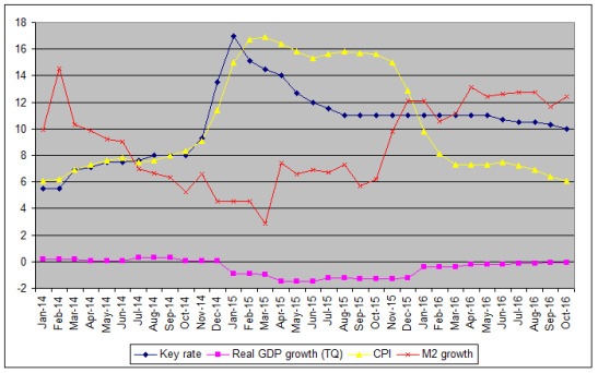
Figure 1. Dynamics of the CPI, key rate, monetary mass M2 and the growth of real GDP (TQ) of Russia during 2014-2016.

Note: M2 growth is marked by a clear seasonal fluctuation in December-January. It was smoothed in the following way: the data for M2 growth for December and January has been averaged, and the resulting average value is used instead of the original values.

The above shows that using the key rate as a tool for stimulating economic growth is a bad idea. This tool does not work. Therefore, in the formulation of monetary policy, a key rate policy cannot be tied to the economic growth plan. A detailed calculation of its impact on economic growth will show that there is no influence.

In this regard, the policy of the key rate should be based not on economic growth but on another indicator that is actually affected by the key rate. This indicator, in our view, is the level of financial stability.

It is clear that the rates affect the level of financial stability of both organizations and the economy as a whole. In addition, it turns out that there are multiple mechanisms of influence:

1. Low rates reduce the interest margin and interest revenue of banks, forcing them to increase lending, and increase the share of speculative transactions and other non-traditional sources of income;
2. Low credit rates do not cover credit risks. However, the banks are forced to keep the rates low because of increased competition from other banks;
3. Lower rates result in financial pyramids in different markets.

Thus, the correlation of the rates with financial sustainability is very strong.

In recent years, owing to the increasing volatility of financial markets, the problems of managing financial sustainability have been the focus of attention of both international financial organizations and central banks in different countries. This has been manifested in the expansion of the regulatory functions of central banks and in the improvement of the regulatory framework, with account for the need to maintain the sustainability of financial institutions and banking systems at an acceptable level. At the same time, the methodology for determining the strategic objective for financial stability and the algorithm for embedding it into monetary policies have not yet been developed.

 The ambiguity of the dependence between economic growth, inflation, and the key rate, on which central banks are relying in modern monetary policy and the necessity of financial stability being included in the monetary policy system in the absence of a methodology requires more detailed study in the following format: “Economic growth – financial stability – price stability – monetary policy”.

3. These studies are complicated by the fact that, as of today, there has been no simple  method for measuring financial stability at the macroeconomic level, even though approaches to measuring the financial sustainability of individual economic agents have been developed a long time ago.

Therefore, we have used real interest rates calculated on different source data as indicators of financial stability.

The grounds for the approach used are as follows:

1. The stability of the economy as a whole can be assessed through the assessment of the sustainability of all core organizations with the subsequent aggregation of results. This approach is hardly possible in real life because it is important not only to provide stability of the organizations themselves, but also the correlation between their risks. It is very difficult to obtain such information, and it is not featured in financial statements.
2. The stability of the economy as a whole can be assessed directly, without the analysis of specific organizations. To this end, it is necessary to investigate the weakest places and the probability of typical crisis scenarios. The history of past economic crises shows that the following accumulated imbalances tend to be the most typical scenarios of crisis development: (1) imbalances between the supply and demand of goods, which are expressed in excess of some goods along with the shortage of others; (2) imbalances between the rate of growth in the prices of individual groups of goods, which usually surpass the increase in the price of resources compared to final products.
3. The above trends, in terms of their causes, have a financial and non-financial component. The financial component is the fluctuation in the supply of money. The non-financial one is various negative factors, such as natural disasters. Given the subject matter of the article, we give our primary focus to the financial component. It affects the economy as a whole, while non-financial factors are very scattered and have a little effect at the macroeconomic level.
4. The impact of money supply on macroeconomic stability is usefully measured by the level of real interest rates. The problem is that almost all the negative effects of the increase in money supply only occur when investors get access to carry-trade, that is, investing in an asset, the rate of price growth of which exceed the borrowing rate. As long as it is possible to make such investments only in financial assets, the situation seems to be acceptable, as high returns on these investments come hand in hand with high risk. However, this risk is borne only by the investors. If the rate falls below the inflation, then such investments can be made in non-financial assets, which will result in the spread of risks across the economy.

These considerations imply that the financial stability is impaired when real rates fall below a level close to zero. It should be noted, however, that the real interest rates are not an indicator of the level of financial stability of the economy at this point in time. They are the leading indicator. Negative effects from low rates should accumulate. This takes a lot of time.

 Here we can observe two types of negative effects – medium and long-term. The medium-term effect consists in the acceleration of inflation caused by an increase in the monetary mass. It starts to show up in about a year. Rising inflation leads to a decline in real income and real GDP. The long-term effect appears in about five years of low-rate policies. It consists of inflating bubbles in different markets – this usually covers securities and real estate; inflating imbalances in investment activity (funds are invested into inefficient, high-risk, or simply useless projects). The short-term effect of low real rates is likely to be positive. It is accompanied by increased demand, while there is still not enough time for negative trends to accumulate.

Therefore:

1. Low real rates are a danger only if they are supported long enough – for a time enough for negative effects to accumulate.
2. The accumulated negative effects are evident at times when the rates are beginning to go up. However, the effects structure depends on the type of effects that have accumulated. If the rates have stayed low for a short period – two to three years, their growth is accompanied by a decline in nominal indicators: salary levels, business profitability, etc. In this case, the reduction is moderate; however, it is not catastrophic. The real figures change insignificantly. If the rates were low for a long period of time, their effects are followed by the collapse of all bubbles, in particular: collapse of stock prices for equities and goods; mass bankruptcies in selected non-financial sectors of the economy; bankruptcy of financial organizations; collapse of real property prices and the associated increase in credit risks; overall growth of credit risk due to various reasons; increase in credit rates due to increased credit risk and liquidity deficit, which additionally amplify the above effects.

The real rate is a generalized concept, since it represents the difference between any nominal rate and any indicator of inflation. The study of the relationship between financial stability and the key rate requires a specification of the real rate concept. To that end, we have used the Index of Financial Stability (IFS), calculated based on official public statements.

The algorithm for calculating this index is represented in following equations (1-5):

IFS = RR = RN – IP,                                (1)

where:

RR is the real average weighted rate of the value of debt financial instruments (borrowings) in percent per year;

RN is the nominal average weighted rate of the value of money (borrowings) in percent per year;

IP is the economic price growth index in percent per year;

RN = (RNC*C + RNB*B)/(C + B), (2)

where:

RNC is the nominal average weighted rate on the loan market in percent per year;

C is the amount of outstanding loans in the credit market in billions of roubles;

CNB is the nominal average weighted rate on the bond market in percent per year;

B is the capitalization of the bond market in billions of roubles;

IP = (Ip * Q + In * N + Ia * А)/(Q + N + А),                                  (3)

where:

Ip is the consumer price index in percent per year;

Q is the real GDP volume in billions of roubles;

In is the consumer price index of the real estate market in percent per annual;

N is the real estate market volume in billions of roubles;

Ia is the stock price index in percent per year;

H is the capitalization of the stock market in billions of roubles;

To calculate parameters RNC and CNB the following formulas were used:

RNC = (RNC1*C1 + RNC2*C2 + RNC3*C3)/(C1+C2+C3),     (4)

where:

RNC1 is the nominal weighted average rate on credits to organizations (excl. credit organizations) in percent per year;

C1 is the amount of outstanding loans (excl. credit organizations) in billions of roubles;

RNC2 is the average weighted rate on credits to credit organizations in percent per year;

C2 is the outstanding debt of credit organizations in billions of roubles;

RNC2 is an average weighted rate on credits to individuals in percent per year;

C3 is the amount of outstanding debt of individuals in billions of roubles;

RNB = (RNB1*B1 + RNB2*B2 + RNB3*B3)/(B1 + B2 + B3),       (5)

where:

RNB1 is the weighted yield of corporate bonds in percent per year;

B1 is the capitalization of the corporate bond market in billions of roubles;

RNB2 is the weighted yield of public bonds in percent per year;

B2 is the capitalization of the public bond market in billions of roubles;

RNB3 is the weighted yield of municipal bonds in percent per year;

B3 is the capitalization of the municipal bond market in billions of roubles.

As we can see from the formula (3), we have made an estimate of the inflation rate, taking into account the changes not only in consumer prices, but also in capital and real estate prices. This is because we use the price index not in a very traditional way – as a measure of the profitability of investment in assets that include goods. Using regular price indices would provide incomplete information. Regardless of the scope of each particular price index base, none of them will take into account the profitability of certain assets. Therefore, the price index was complemented by yield of the assets, which are the most likely to create bubbles.

As for the choice between the CPI and the GDP price deflator, the latter is in favor due to its broader base of calculation. However, the low rate of statistics updates is a significant drawback, which determines the choice of the CPI. In addition, numerically GDP deflator and CPI differ insignificantly.

Figure 2 illustrates the comparison of the proposed IP index with CPI in the context of the Russian economy. Figure 2 shows that the CPI curve does not coincide with the overall inflation index curve. The overall inflation index is changing more dynamically than CPI and responds faster to crises. For the majority of the period analyzed, it was below CPI. With the exception of the periods from September 2014 to February 2015 and from September 2016 to October 2016. The lower level of overall inflation can be explained by the higher decline in real estate and capital prices than in consumer goods during the crisis.

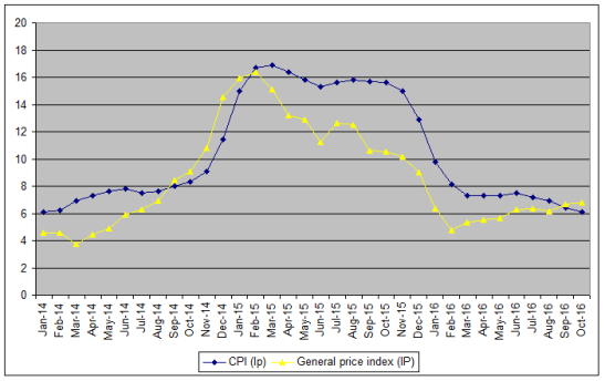
Figure. 2. Dynamics of the General Inflation Index (IP) and CPI (Ip)

The following algorithm for calculating the Index of Financial Stability (IFS) was tested on the statistical data for Russian Federation for 2014-2016.

Due to the lack of public access to official records containing statistical information on a number of indicators used in equations (2-5), we have made the following assumptions when calculating the Index of Financial Stability:

1. The bond market data were evaluated for three markets: corporate, public, and municipal bonds markets. A convenient source of information is the bond returns indices, which are calculated by the Moscow Exchange:

• “Corporate Bond Index” [9]
• “Municipal Bond Index” [10]
• “Public Bond Index” [11]

The main index parameter is the average yield of the corresponding bonds, while the secondary parameter is their capitalization. The historical data for public bonds are incomplete: Capitalization is given only for the last month (December 2016), and the return data is available starting June 2015. The missing data were calculated as follows:

• Return on public bonds is equal to the profitability of municipal bonds minus 1.23% (this number is defined by comparing the profitability of municipal and state bonds from the time when the profitability data became available for the public bonds as well).
• Capitalization of the public bonds market is calculated based on the internal public debt data published on the website of the Ministry of Finance [12] and the share of the bonds in the total debt. The share of the bonds amounted to 57.9%. It was estimated based on the capitalization of the market bonds at 3472 billion roubles in December 2016 and the internal public debt (minus guarantees) at 5994 billion roubles on the same date.

2. The total amount of outstanding shares (free flat) was used as a weight index for the stock market. The rate of turnover was not considered objective. It is highly overstated due to a large number of short-term transactions. Free float was calculated by multiplying the capitalization of shares and the percentage of outstanding shares (free float index). This information is published on the website of Moscow Exchange [13, 14].
3. Real estate prices were determined based on the statistics for the city of Moscow [15], since this information is the most reliable and is regularly updated. We suppose that the real estate price dynamics should match that of Moscow, although the absolute level of prices in the regions is lower.
4. The volume of real estate transactions was calculated based on the data of Rosreestr (Federal Service for State Registration, Cadaster and Cartography) by multiplying the number of registered property rights [16], the average size of the real estate object (assumed to be equal to 50 sq.m.) and the average price per square meter (the price of real estate in Moscow on the corresponding date reduced by 2 times).

The results of the calculation of the Index of Financial Stability and its monthly dynamics for the period from January 2014 to October 2016 are presented in Figure 4.

 

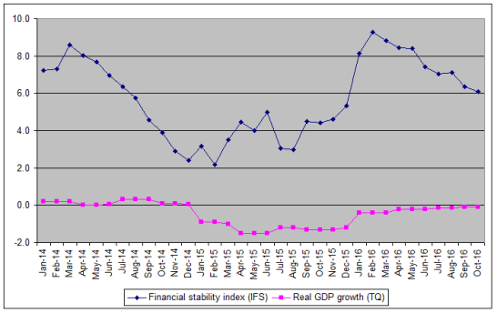
Figure. 3.  Dynamics of the Index of Financial Stability (IFS)

and real GDP growth (TQ).

The graph shows a smooth decline of IFS in 2014. At the same time, the real GDP growth rates did not respond to such decline for nine months. Since 2015, there has been a sharp decline in real GDP growth. The reason for the decline was the increased inflation. The cause of inflation was the soaring of foreign exchange rates (rouble depreciation) in the 4th quarter of 2014. There were two reasons for rouble depreciation: excess of monetary mass compared to the accumulated gold and foreign currency reserves and liquidity problems in world financial markets in 2014, which made it difficult for Russian companies to refinance foreign loans. It should be noted that in 2014, M2 was not growing, but declining, and this occurred against the increase in the key rate (Figure 1). These two trends can lead to a false assumption that the Bank of Russia pursued a rigid monetary policy, which makes the acceleration of inflation unlikely. However, IFS was going down, indicating the accumulation of problems in the economy.

Since the beginning of 2015, IFS was growing very slowly, with the acceleration in 2016. The dip in the real GDP almost disappeared by the Fall of 2016. This shows that there is approximately a one-year lag between the changes of IFS and of the real GDP growth.

Based on the arguments presented above, we perceive IFS as a very useful leading indicator, which illustrates the processes of reducing or increasing the financial stability of the economy. This raises the question as to what level the IFS can drop until it becomes unacceptable.

This level can be set based on the following considerations:

1. IFS can help predict a decline in financial stability caused by the formation of bubbles/pyramids and the accumulation of subsequent negative effects. IFS does not detect the other risk growth mechanisms, but they are less important.
2. The bubbles are always formed in specific markets or in certain areas of activity. It follows that in order to monitor the situation in the most important fields one should apply private IFS and demand that each of them stays above a minimum value. We propose to use the indices calculated using formula (1) as a private IFS, which instead of the general IP price index, use the private price indices Ip, In, Ia from formula (3). If necessary, the list of private IFS can be expanded by using price indices for other asset groups.
3. The general IFS characterizes the situation as a whole. It requires the introduction of a minimum threshold with a certain leeway.
4. Considering the above analysis of the Russian situation, in the Russian context, it would be reasonable to set the minimum value for private IFS at 1%, and set the minimum for overall IFS at 3%. This is shown in more detail in table 1. It also contains criteria for high stability, which ultimately results in three levels of stability: low (negative zone), medium, and high.

 Table 1

Scale of stability levels

Level of stability	General IFS	Private IFS
High	IFS ³ 6%	IFS³4%
Medium	3%£ IFS<6%	1%£ IFS<4%
Low	IFS<3%	IFS<1%

Maintaining the IFS at a high level is a difficult task. The following are the main issues, which have to be addressed:

1. As it has already been mentioned, the increase in IFS increases the likelihood of a financial crisis, if before the increase the IFS was low in a negative zone. Therefore, one has to increase the IFS from lower levels very slowly and gradually, addressing the new issues after each step.
2. In order to achieve stability, IFS should be maintained at a high level for a long time. Accordingly, the increase of IFS should be based on the developed strategy. Utilizing IFS increase to achieve some tactical objectives is useless. On the contrary, IFS can be decreased in order to resolve the short-term liquidity crises. This applies only to short-term crises, however.
3. High IFS makes it difficult to resolve problems that require liquidity. These include financial recovery of organizations, including bank sanation; providing regular payments during the shortage of monetary resources in corresponding funds; financing unforeseen public expenditures.
4. High IFS complicates the resolution of budgetary problems. Covering the budget deficit by the emissions will lead to an increase in the supply of money and reduce the IFS below the planned level. Covering the deficit through borrowing will be cost-intensive due to high rates. At the same time, it will draw money out of the economy.

The above shows that the impact of IFS on the economy does not depend on monetary policy. IFS is an independent variable. Therefore, the government can fix it at the proper level and continue further development of the key rate policy, taking into account the set level of IFS.

The nominal rate (RN) can be expressed from a formula (1):

RN = IFS + IP,                              (6)

On the other hand, the nominal rate can be presented as the sum of the risk-free rate and the risk premium:

RN = RNF + RNR              (7)

where:

RNF is the nominal risk-free rate,

RNR is the risk premium.

If the key rate (r) is used as a risk-free rate, it can be calculated from equations (6) and (7):

r = IFS + IP – RNR   (8)

In formula (8), we should use the target value of the Index of Financial Stability for the coming period as the IFS. For Russia, the target value of the IFS should be calculated based on the criteria provided in Table 1. This value is expected to change smoothly, or remain at a constant level. We should also use a realistic forecast of price growth and not a planned value as the IP. It is useful to calculate the RNR risk premium based on the statistics for the previous periods. Let us explore in more detail the behavior of the RNR risk premium. Figure 4 shows a graph of the dynamics of the RNR risk premium in Russia, which was calculated as a difference between the average weighted nominal rate and the key rate. Figure 4 shows that RNR is declining very smoothly. This reduction can be easily approximated using the linear time dependence. The correlation here is rather strong – the coefficient R² = 0.7141, the coefficient of linear correlation R = –= – 0.845.

In the linear dependence equation chart, x stands for the date (number of the month starting from January 1900). If we take January 2014 as a zero point, the equation will look as follows: y = 5.509-0.0906 x.

Thus, the key rate will be linked to three indicators, two of which (IFS and RNR) are fixed in the short term, and the third (IP) is changing.

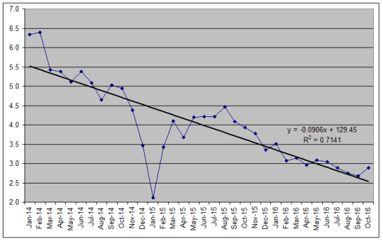
Figure. 4.  The risk premium in Russia from 2014 to 2016.

The reason for this smooth decline of RNR is that, in 2014, the Bank of Russia canceled the refinancing rate and switched to targeting market rates. At the same time, the key rate has become the target for market rates, which leads to their gradual convergence. According to our assessment, the reduction of RNR will stop at 2-2.5%. It will not reach zero, because the Bank of Russia targets the rates using low-risk instruments rather than aims at the market average. Therefore, for further calculations we are going to assume that the value of RNR = 2%.

 

4. Some practical aspects of the application of the financial stability-targeting regime will be discussed in the monetary policy of the Bank of Russia, adopted for the period 2017-2019. To this end, let us calculate the values based on IFS and the key rate for the same period using the methodology proposed above.

In order to calculate the strategic objectives in the new format, we used the information from the Bank of Russia on scenario forecasts of the real GDP growth rate and the CPI in the planned period [17]. At the same time, we used the values of the standard scenario as the starting point (table 2).

Table 2

Source information (base version of scenario forecast)

	2017	2018.	2019
Real GDP growth rate, %	0,5-1,0	1,5-2,0	2,0-2,5
CPI,%	4.0	4.0	4.0

As you can see from the Table. 2, the Bank of Russia adopted a 4% CPI as a strategic goal for inflation. However, the GDP growth forecast was defined in the range (0.5-1.0)% in 2017, (0.5-2.0)% in 2018, and (2.0-2.5)% in 2019.

Based on the strategic goal of GDP growth, we set the target value of IFS, corresponding to the positive economic growth rate at 6%, 6.1% and 6.2% respectively. The strategic objective for financial stability in 2017 was established in the light of the current level of financial stability as of the end of 2016 (6.1%) and acceleration of the real GDP growth. However, the growth of the Index of Financial Stability included minor year-to-year changes in order to avoid creating threats to the state of the financial market.

The expected level of the key rate was calculated as the sum of the Financial Stability Index and the Price Stability Index (IP) minus the RNR risk premium. The target-level (IP) calculation has, however, taken into account the CPI goal of 4.0 percent in each year and the trend of IP exceeding the CPI (Figure 2), which came about in the end of 2016.

The results of the calculation of the strategic objectives for the level of financial stability under the base option are presented in Table. 3.

Table 3

Strategic objectives of monetary policy (base scenario)

	2017	2018.	2019
Index of Financial Stability (IFS)	6.1	6.2	6.3
Price Stability Index (IP)	4.5	4.5	4.5
Including Price Stability Index (CPI)	4.0	4.0	4.0
Risk Premium (RNR)	2.0	2.0	2.0
Key rate	8.6	8.7	8.8

As you can see from the Table. 3. in the medium term, the strategic objective for financial stability should most likely be defined at 6.1% in 2017, 6.2% in 2018, and 6.3% in 2019. In such a case, the key rate should stay in the range of 8.6% – 8.8%.

The presented algorithm for calculating monetary policy objectives in the new format was used to define the goals in the light of the different scenarios of economic development. The results of these calculations are presented in Table. 4.

Table 4

Strategic objectives of monetary policy in different scenarios,%

Objectives/ Scenarios	2017			2018.			2019
	Base	Pessimistic	Optimistic	Base	Pessimistic	Optimistic	Base	Pessimistic	Optimistic
Index of Financial Stability (IFS)	6.1	3.5	6.2	6.2	5.5	6.5	6.3	6.2	6.5
Price Stability Index (IP)	4.5	6.0	4.5	4.5	4.8	4.5	4.5	4.5	4.5
Including Price Stability Index (CPI)	4.0	5.5	4.0	4.0	4.3	4.0	4.0	4.0	4.0
Risk Premium (RNR)	2.0	2.0	2.0	2.0	2.0	2.0	2.0	2.0	2.0
Key rate	8.6	7.5	8.7	8.7	8.3	8.5	8.8	8.7	9.0
Real GDP growth rate *	0,5-1,0	-(1,5-1,0)	1,2-1,7	1,5-2,0	-(0,5-0,1)	2,0-2,5	1,5-2,0	1,3-1,7	2,0-2,5

* for reference

Table 4 shows that, in the face of an adverse external environment, the strategic objective for financial stability is adjusted to 3.5% in 2017, 5.5% in 2018, and 6.2% in 2019. In such a case, we should expect the minimum level of the key rate to be 7.5% (2017) and the maximum – 8.7% (2019). If the economic conditions are more favorable than the basic option, the Financial Stability Index will be in the range (6.2-6.5)%. At the same time, the key rate will reach 9.0% by the end of the medium-term period.

5. The conducted studies lead to the following conclusions:

1. In the key rate policy, targeting financial stability is more appropriate than targeting inflation.
2. The Index of Financial Stability proposed in the article is the leading indicator of the change of financial stability.
3. The target value of the Financial Stability Index should be determined based on the levels and criteria of stability established in the context of the country’s economy. It should be positive, exceed the minimum acceptable level, and avoid abrupt changes.
4. For targeting financial stability, the key rate should change in such a way that the Financial Stability Index remains at the targeted level.
5. The benefits of the financial stability-targeting regime are as follows: enhanced coherence between the monetary, economic, and debt policies of the government; increased objectivity and predictability of management decisions of central banks; increased information value of the of monetary policy direction indicator; improved quality control of monetary policy.
6. The proposed methodology for targeting financial stability is universal and can be applied to the activities of central banks in different countries.

6. References

1. Glazyev S., Ivanter V., Makarov V., Nekipelov A., Tatarkin A., Grinberg R., Fetisov G., Tsvetkov V., Batchikov S., Ershov M., Mityaev D., Petrov Yu. (2011). On the strategy of economic development of Russia. Ekonomicheskaya Nauka Sovremennoi Rossii, No. 3, pp. 1—26. (In Russian).
2. Manevich V. (2010). On the role of monetary and fiscal policies in Russia at the crisis and post-crisis periods. Voprosy Ekonomiki, No. 12, pp. 17—32. (In Russian).
3. Rudebusch G., Svensson L. (1999). Policy rules for inflation targeting. In: J. B. Taylor (ed.). Monetary policy rules. Chicago: University of Chicago Press, pp. 203—246.
4. Giannoni M., Woodford M. (2003). Optimal interest-rate rules: II. Applications. NBER Working Paper, No. w9420.
5. Giannoni M., Woodford M. (2004). Optimal inflation-targeting rules. In: The inflation-targeting debate. Chicago: University of Chicago Press, pp. 93 — 172.
6. Blanchard O., Gali J. (2010). Labor markets and monetary policy: A new Keynesian model with unemployment. American Economic Journal: Macroeconomics, Vol. 2, No. 2, pp. 1-30.
7. Schmitt-Grohe S., Uribe M. (2007). Optimal simple and implementable monetary and fiscal rules. Journal of Monetary Economics, Vol. 54, No. 6, pp. 1702 — 1725.
8. Moiseev S.R. Rules for monetary policy / Finance and credit, #16-2002, pp.37-46. (http://www.mirkin.ru/_docs/articles03-019.pdf).
9. MICEX Corporate Bond Index MICEXCBITR – historical data // Moscow Exchange – URL: http://moex.com/en/index/MICEXCBITR/archive/.
10. MICEX Municipal Bond index MICEXMBITR – historical data // Moscow Exchange –URL: http://moex.com/en/index/MICEXMBITR/archive/.
11. Russian Government Bond Index RGBITR – historical data // Moscow Exchange – URL: http://moex.com/en/index/RGBITR/archive/.
12. Russian Federation state domestic debt – monthly data // Ministry of Finance – URL: http://minfin.ru/ru/document/?id_4=93479.
13. Moscow Exchange stock market capitalisation data // Moscow Exchange – URL: http://moex.com/a3882.
14. Stock market free-float coefficient data // Moscow Exchange – URL: http://moex.com/ru/listing/free-float.aspx.
15. Reality price statistics for Moscow city // URL: http://www.irn.ru/gd/.
16. Federal Service for State Registration, Cadaster and Cartography statistics // URL: https://rosreestr.ru/site/open-service/statistika-i-analitika/statisticheskaya-otchetnost/.
17. Guidelines for the Single State Monetary Policy // Bank of Russia – URL: http://cbr.ru/eng/publ/?PrtId=ondkp.

Authors

Galina Gospodarchuk is Doctor of economics and Professor of the Department of Finance and Credit Lobachevsky State University of Nizhni Novgorod- e-mail: gospodarchukgg@iee.unn.ru

Sergey Gospodarchuk, PhD in economics, is Individual researcher – e-mail: sergeyg1@yandex.ru